How occlusion structure breaks CNN digit recognition
- 6 minsThe motivation for this post is the following
This post is about that difference.
I wanted to test a simple question: when a CNN fails under occlusion, is it mainly because too much information is gone, or because the missing information has the wrong spatial structure? In other words, are random pixel dropouts and smooth, contiguous occluders equally destructive if they remove the same number of pixels?
To make the question clean, I used a deliberately small and canonical benchmark: MNIST, wrapped into a Moving MNIST setup. MNIST is tiny, fast, ubiquitous, and almost boring — which is exactly why it is useful here. If a pattern already appears on handwritten digits, then it is likely to reflect something real about the model rather than some unnecessary complexity in the dataset.
The results (to be seen) are straightforward and, I think, quite instructive. What is interesting is how clearly it shows up, not only in accuracy, but in confidence and calibration as well.
The setup
Moving MNIST takes a digit and lets it move across a larger canvas over time. That gives a toy video task instead of a static 28×28 classification problem.
Here’s an example of what that looks like
I train the model on such clean frames, then evaluate it on occluded videos, aggregating predictions across a few frames. That way the experiment is still lightweight, but not completely trivial: the model gets multiple glimpses of the same digit, just as a human observer might.
CNN architecture
Here is the architecture used for the classifier:
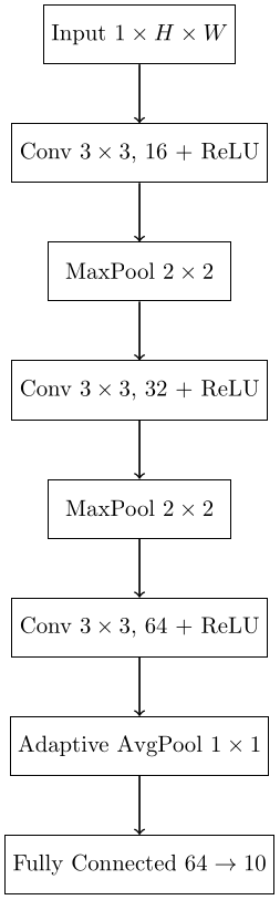
Nothing exotic is happening here. This is a small convolutional network with pooling and a final linear classifier. The point is not to squeeze out state-of-the-art performance, but to probe a standard CNN in a controlled setting.
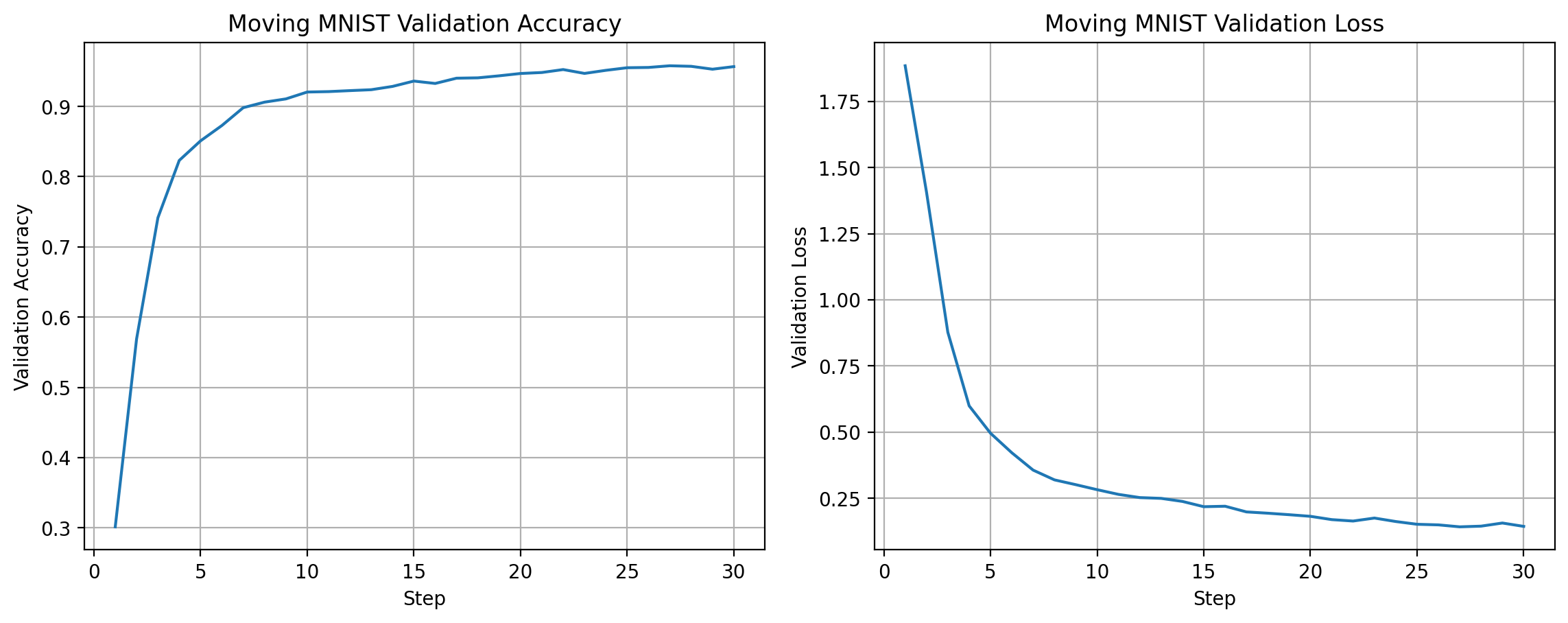
The training dynamics look as expected: accuracy rises rapidly (until around 95%) while the validation loss falls and stabilizes after a few epochs.
Occlusion models
The occlusion families are the real protagonists. I used four of them:
- Bernoulli masks, where each pixel is independently dropped.
- CGOL masks, formed by evolving random binary patterns with Conway’s Game of Life.
- Triangular masks, made from a small number of polygonal occluders.
- Perlin-style masks, generated from smooth spatially correlated noise.
Why these four? Because they span the spectrum from unstructured to strongly structured. Bernoulli dropout is the classic “missing at random” baseline. Perlin and triangular masks create coherent holes, much closer to what we usually mean by occlusion in the real world. CGOL sits somewhere in between: clustered and structured, but less geometric.
The difference is immediately visible:
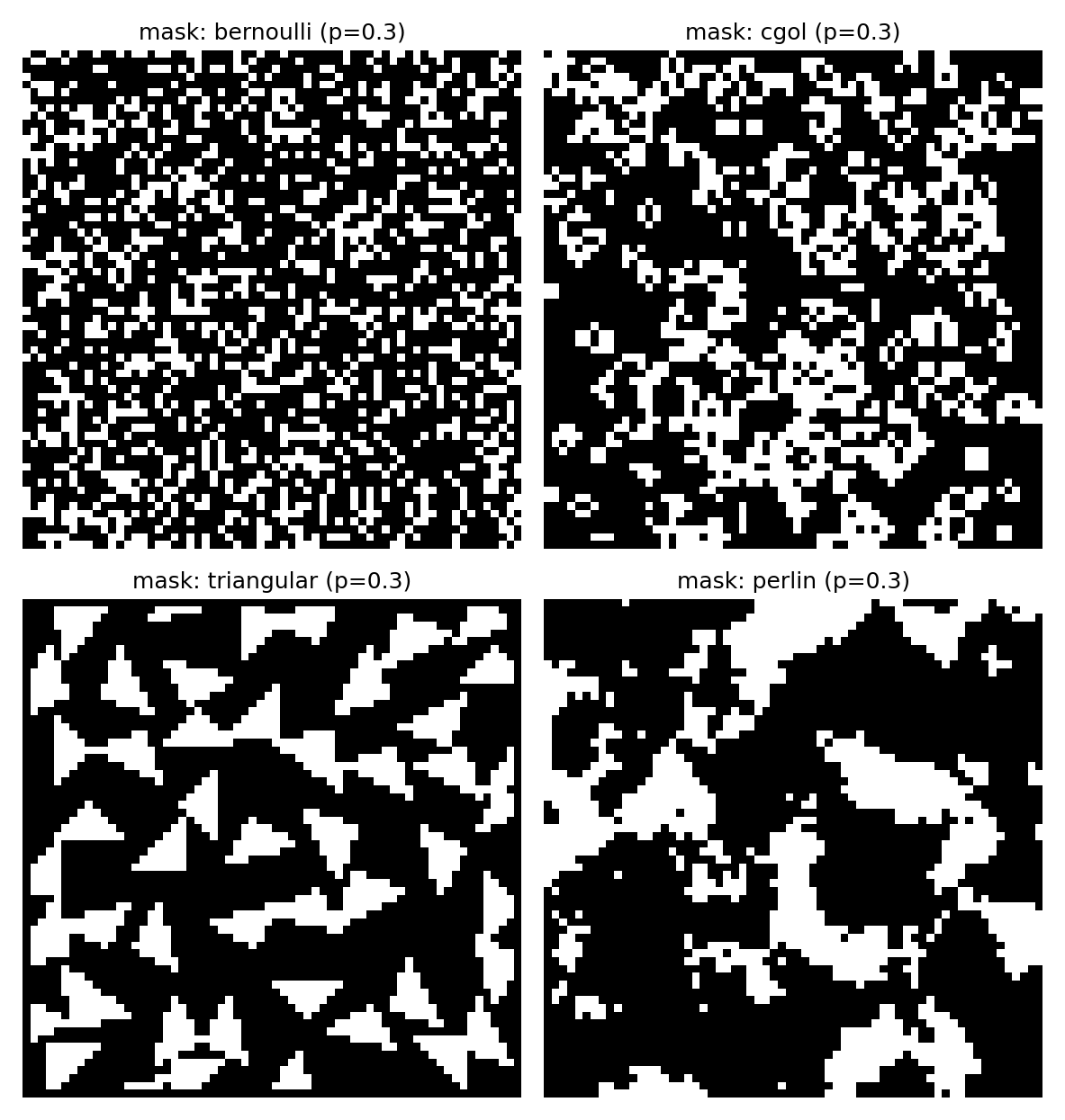
Even when the overall coverage is matched, these masks do not remove information in the same way. Bernoulli leaves tiny holes everywhere. Perlin and triangular masks erase connected chunks. That distinction turns out to matter a lot.
A visual example
Before showing aggregate plots, it helps to look at one concrete sequence. In the following video, the same Moving MNIST digit is shown side by side under two different occlusions: Bernoulli on one side, Perlin-style on the other.
The Bernoulli version is noisy, but still legible. The stroke structure survives in lots of little fragments. The Perlin version is different: whole pieces of the digit disappear together. The digit can stop looking like itself even though the total fraction of missing pixels is comparable.
That is the qualitative intuition. The rest of the experiment is about measuring it properly.
What is measured
The main metric is video-level accuracy: after running the CNN on several frames, I aggregate its log-probabilities and ask whether the final video prediction is correct. This is the natural end task.
But accuracy is not the whole story, so I also track the model’s probability estimates.
If the model assigns probability $p(y_{\mathrm{true}})$ to the correct class, then the negative log-likelihood is
\(\mathrm{NLL} = -\log p(y_{\mathrm{true}}).\)
Lower is better. NLL becomes large when the model is confidently wrong or simply fails to allocate much mass to the true class.
The Brier score measures the squared error of the full probability vector against the one-hot label,
\(\mathrm{Brier}(p,y) = \sum_i (p_i - y_i)^2,\)
so it mixes together accuracy and probability quality.
Finally, there is ECE, the expected calibration error. This tells us whether confidence is actually trustworthy: if a model says “I am 80% confident”, is it right about 80% of the time? Large ECE means the confidence values are not lining up well with reality.
Since the whole point of the experiment is to compare occlusion geometry, I also compute structural descriptors of the masks themselves: realized coverage, the size of the largest connected occluder, and the number of connected components.
Results
The main figure is enough to see the whole story:
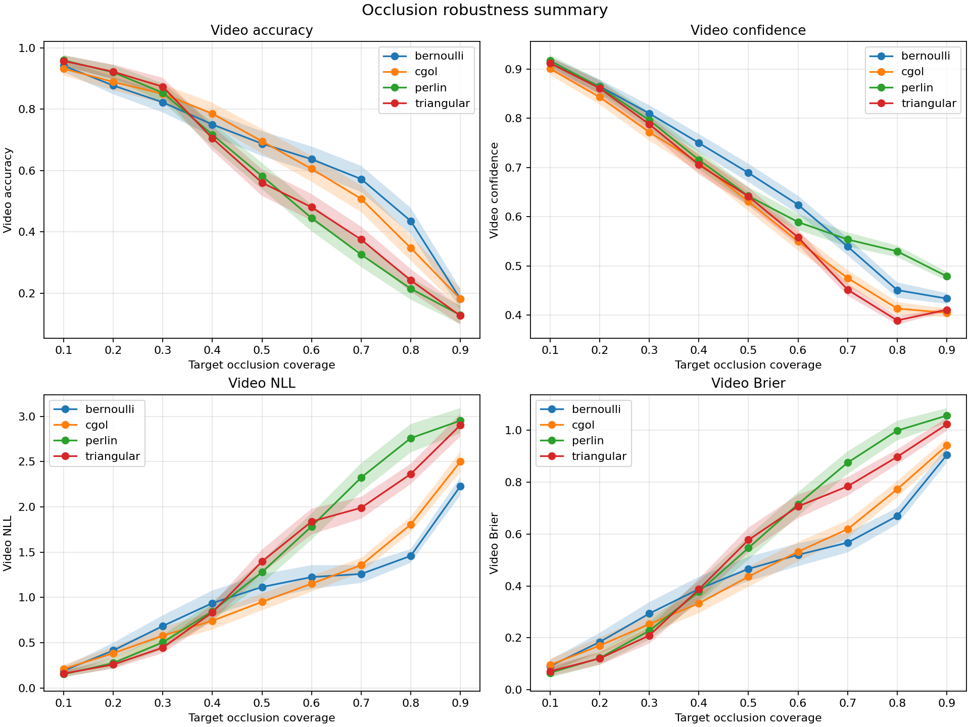
As coverage increases, performance drops for all mask families. That part is unsurprising. What matters is the ordering. Bernoulli degrades the most gracefully. CGOL is worse. Perlin and triangular masks are clearly the most destructive.
This means that “50% occluded” is not a complete description of the input. Two masks can remove the same fraction of pixels and yet produce very different recognition behavior. A scattered pattern of missing pixels is much easier for the CNN to tolerate than a connected region that wipes out an entire stroke.
That same pattern appears in the probability metrics. Perlin and triangular masks give the worst NLL and Brier scores, which means they do not just reduce top-1 accuracy — they damage the model’s belief state more broadly. The classifier becomes worse at assigning sensible probabilities, not merely worse at picking the argmax.
Calibration also degrades in a meaningful way:
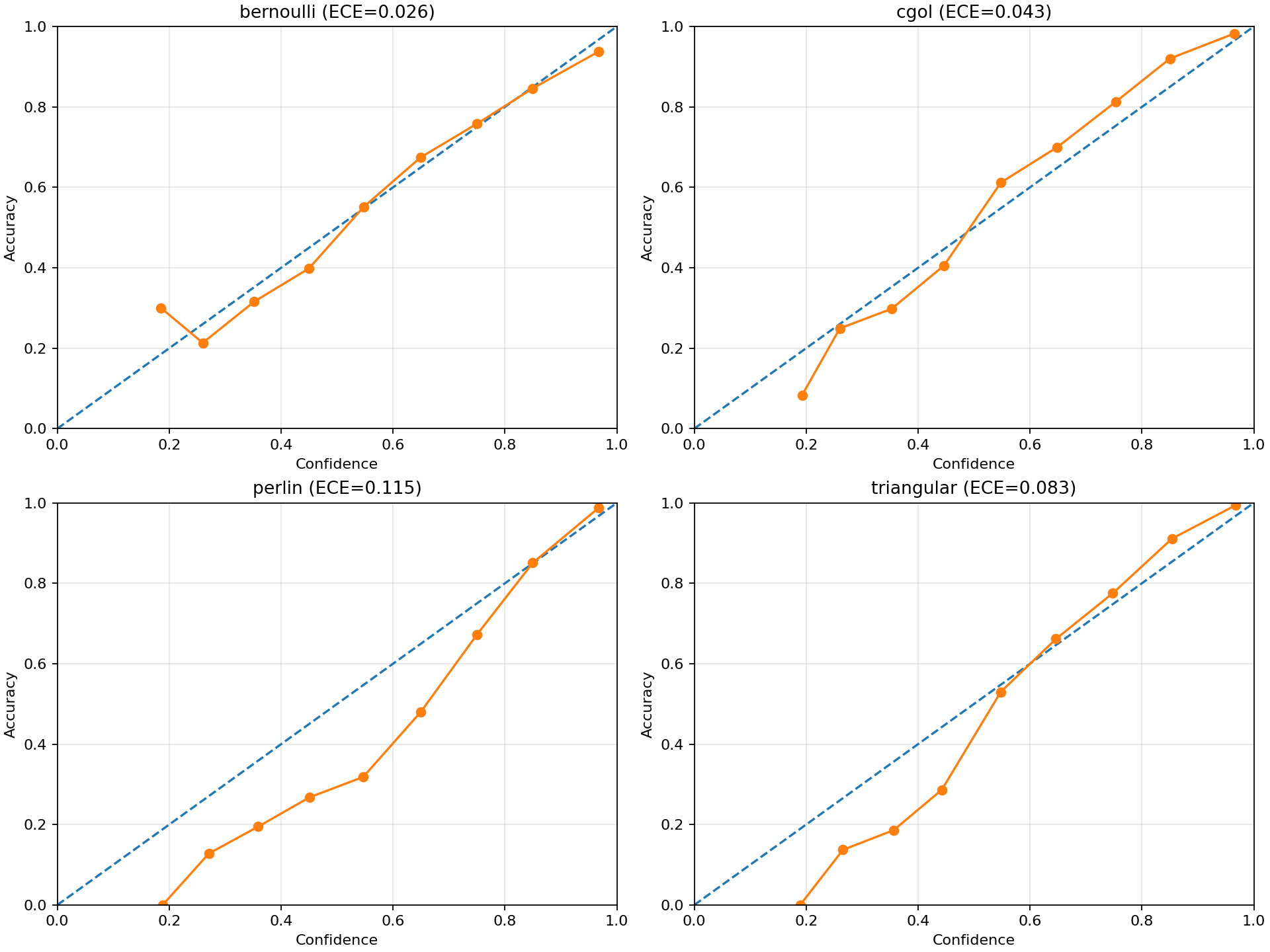
This plot is especially useful because it shows that robustness is not just about accuracy. Under structured occlusion, the model’s confidence becomes a less reliable guide to correctness. In other words, the classifier is not only more likely to fail — it is also less honest about how uncertain it should be.
Conclusion
Occlusion does not just depend on how much information is removed, but how it is removed. Random pixel dropout spreads small gaps across the image, which a CNN can often tolerate because local evidence remains available. Structured occlusions, in contrast, remove coherent chunks of information and degrade the representation much more abruptly.
This highlights a limitation of common robustness benchmarks. Many rely on iid noise or dropout-style corruption, which does not reflect how occlusion typically appears in real scenes. As a result, a model can look robust under random masking while still failing under structured occlusion.
Even in a tiny setting like Moving MNIST, the distinction is clear: geometry matters.