Motion computation via an unsupervised-learning approach (pt.1)

This new blog-post series is about how seemingly-distant fields (computer-vision, audio) and their underlying principles (deep-learning vs. DSP) come together, through my (and everyone’s) favorite mathematical concept: the Fourier Transform (see first and second blog-posts). This first part will introduce a novel approach for computing motion in occluded videos, and build the foundation from which we will cross the threshold into the Fourier (complex) domain and its associated operators, doing this a step at a time.

First though, a little introduction.

Intro

Motion computation and fragmented occlusion

For those who don’t know: I (not so) recently started a PhD in computer vision in Vienna, and was immediately thrown into a niche problem not many people are currently focusing on: that of estimating the motion of objects in occluded scenarios. While there are various types of occlusion out there, I am mainly focusing on fragmented occlusion, whereby occluders potentially create individually unrecognisable fragments of an object (think of this Magritte painting, had he chosen less recognisable body-parts).

For the case of motion computation under fragmented occlusion, think about describing this squirrel’s movement (put some death metal in the background instead of that annoying music).

More specifically, within the first 10 seconds of this video, in approximately how many frames (if any) can the squirrel be seen in full?

While general algorithms for motion computation have been in existence since the 1980’s, these algorithms are usually built on underlying assumptions which don’t really hold in occluded scenarios (to understand why- read more about the brightness constancy assumption). Thus, a different set of computational tools is necessary for computing motion in the occluded case. I’ll try to briefly present these tools, and get on to the more interesting stuff.

Parametric motion models

Working in the occluded case demands a simplified motion, i.e. we begin with a global parametric-motion model assumption over all pixels in the image instead of assuming that local neighborhoods move coherently, with smooth variation in motion across the entire image. This motion depends on an initial number of parameters, which are used at each time-step to successively warp some initial frame, thus creating a motion video.

The simplest such example is a translation model, equivalent to using one finger to move a widget across your mobile-phone desktop. Somewhat more elaborate motions can be modelled via rotation (3DoF = translation + rotation), similarity (4DoF: translation+rotation+scale), affine (6DoF- all previously mentioned + shear) motion models, and even projective (9DoF) where each of these transformations have different geometric invariants. for example: a similarity transformation preserves shape up to a scalar, whereas an affine motion model need not necessarily retain shape, but rather preserves parallel lines (a square may morph into a parallelogram), and the ratios of lengths of parallel line segments.

See this example for a synthetic 6DoF affine motion video featuring a moving soccerball-like object. Notice that it moves towards the bottom-right corner, rotating counter-clockwise and eventualy deforming into an elongated ellipsoid (shear is non-zero).

Motion computation via an unsupervised-learning objective

An effective algorithm for motion computation in occluded videos has already been thought up, developed and patented by my PhD supervisor Dr. Roman Pflugfelder (may he live long!). So far the algorithm works well for computing 1D-horizontal (very simple) motion, as well as reconstructing hidden moving objects in heavily-occluded videos, but doesn’t work well in the higher-dimensional case. This algorithm is now briefly presented

Inputs:

• Video frames $ I_0, I_1, \dots, I_{T-1} $, where $ I_{0<=j<=T-1} $ is an image of dimensions $HxW$

Output:

• Optimal motion parameters $ \theta^\star $

Step 1 — Initialize

Initialize motion parameters:

for a $K$-dimensional parametric motion model.

Step 2 — Warp Frames

For each timestep $t = 0, \dots, T-1$:

1) Warp the frame $I_t$ using the current motion parameters:

2) The composite warp $W^t$ is defined as a composition of $t$ successive warps:

Note: Depending on the motion model, the composition $W^t$ can often be simplified analytically (e.g., when motion transformations form a group). Think of applying a shift using parameters $\theta=[\tau_x, \tau_y]$ n times being equivalent to a single shift with parameters $\theta_n=[n \tau_x, n \tau_y]$.

Step 3 — Integrate Warped Frames

Integrate the warped frames into a single averaged image:

Step 4 — Optimization objective

Define the optimization objective as the variance over the integrated image $\overline{I}$:

Note: If we could model the warp operator $W^t$ as multiplication by an exponential scalar $r^t$ (hint: what if $r \in \mathbb{C}$, or even $r=e^{-j \omega}$?), we could represent the summation term in a closed analytical form, thus making our life much easier (more on this in the next blog post).

Step 5 - Optimize over motion parameters

Solve for

using a numerical optimization method (e.g., gradient ascent/descent), with backpropagation through the warp operator $W$, updating $\theta$ at each iteration.

Intuition

The ground-truth motion parameters $\theta^\star$ should yield an integrated image $\overline{I}$ with $maximal$ variance (meaning maximum image contrast). The reason why this algorithm works well in the case of fragmented occlusion is because occlusion is in essence “smoothed” out by the integration procedure, thus leaving only a sharp image of the object in motion, notwithstanding certain assumptions about object visibility across all frames, static occluders, etc… In the next blog-post we will go more into depth with this algorithm, gaining another interpretation of our objective, namely the variance of the integrated image, through the Fourier Transform and the equivalent operator in the Fourier-domain.

Optimization in practice

We will work with a simple toy example: computing the shifting motion of a white rectangle within an unoccluded black background.
Let’s begin by getting some visual info as to how the different concepts look.

Integration

Suppose our image is of a white square centered within an unoccluded black background, and we choose a 2D translation motion model $\theta=[\tau_x, \tau_y]$, where at each step we shift the square towards the top-left corner (non-zero negative values for both $\tau_x, \tau_y$). Here’s some code to generate such an image, as well as a motion video from the image and input shift parameters.

Note: the implementation is differentiable, namely uses only differentiable functions for which the gradient can be computed using Pytorch’s native auto-differentiation engine. This is crucial for optimization to work.

import torch
import torch.nn.functional as F

def make_image(image_dims):  
    """
    Create a base image from which to create a motion video, depending on shape input
    """
    B, H, W = image_dims
    max_dim = max(H, W)
    margin = max_dim//5
    # image is drawn within these bounds, leaving an image border of padded zeros 
    bounds = slice(margin, max_dim - margin)
    # Create a batch of images (B, 1, M, N)
    frames=torch.zeros(B, 1, H, W)
    # white square
    frames[...,bounds, bounds] = 1
    return frames, bounds
    
def shift_motion_vids(motion_vid, shifts):
    """
    Shift successive frames of a motion video using shift parameters.
    """
    B, T, H, W = motion_vid.shape

    shifted = torch.zeros(B, T, H, W, device=motion_vid.device)
    
    # Correct normalized grid
    grid_y, grid_x = torch.meshgrid(torch.linspace(-1, 1, H, device=motion_vid.device), 
                                    torch.linspace(-1, 1, W, device=motion_vid.device), indexing='ij')
    # flipped for grid_sample
    grid = torch.stack((grid_x, grid_y), dim=-1).unsqueeze(0).expand(B, H, W, 2)
    
    # can vectorize this
    for t in range(T):
        cur_shift = t*shifts
        cur_frame = motion_vid[:,t,:,:].unsqueeze(1) #(B, 1, H, W)
        shift_x = 2 * cur_shift[:, 0] / (W - 1)  # normalize to [-1, 1], (B, @)
        shift_y = 2 * cur_shift[:, 1] / (H - 1)
        # Create flow grid for this frame
        flow_grid = grid.clone() #(B, H, W, 2)
        flow_grid[..., 0] -= shift_x.view(B, 1, 1)  # Shift x coordinates
        flow_grid[..., 1] -= shift_y.view(B, 1, 1)  # Shift y coordinates
        warped = F.grid_sample(cur_frame, flow_grid, align_corners=True, 
                              mode='bilinear', padding_mode='border')
        shifted[:, t, ...] = warped.squeeze(1)
    
    return shifted


def spatial_pipeline(motion_vid, shifts, dims = (-2, -1)):
    """
    Whole pipeline in spatial domain: warp motion video frames, integrate warped frames, 
    compute variance over integrated image
    """
    shifted = shift_motion_vid(motion_vid, shifts)
    integrated = shifted.mean(dim=1).unsqueeze(1)
    variance = integrated.var(dim=dims)
    # Return all intermediate variables
    return shifted, integrated, variance

We use this code to compute integrated images for two different input shift parameters as follows

#reproducibility
torch.manual_seed(0)

# image dimensions
B = 2  # Batch size
H, W = 128, 128  # Image dimensions
T = 5  # Number of frames in motion video
SHIFT_SCALE = max(H, W)//(5*T*B) # don't want shape to leave margin within T steps

# Define shifts (for example, shift by (5, 3) for each sample in the batch)
shifts = (torch.arange(-B, B).reshape(B,2)) * SHIFT_SCALE # shape (B, 2)
image_dims = B, H, W
frames, bounds = make_image(image_dims)

# Create motion videos by applying shifts to a 'static' video
static_video = frames.unsqueeze(1).expand(B, T, H, W)
motion_video = shift_motion_vids(static_video, T, shifts)
# Create integrated image with zero shift from motion video 
_, integrated_zero, _ = spatial_pipeline(motion_video, T, torch.zeros_like(shifts))
# compute ground-truth integrated image of original square by 'undoing' motion
theta_star = -shifts 
_, integrated_gt, _ = spatial_pipeline(motion_video, T, theta_star)

Compare now the two integrated images, with shift parameters $\theta=[0, 0]$ and ground truth shift parameters $\theta^\star$.

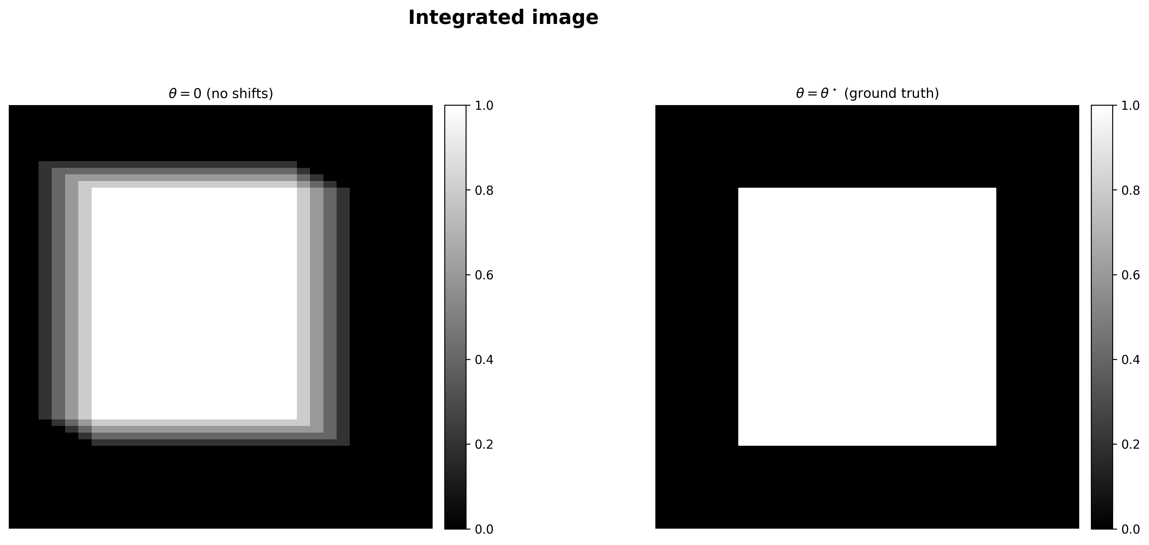
Which of the two images will yield larger variance, and why?

Optimization using pipeline

We now show how to use our full pipeline for optimization over shift parameters, solving for motion.

# estimated shifts should be within this distance from GT for successful optimization, equivalent to 1 EPE (end-to-end point error)   
SUCCESS_THRESH = 1/T

def compute_motion(videos, max_steps=400, thresh=SUCCESS_THRESH, num_trials=T):
    """
    Compute motion via optimization over videos using spatial pipeline. 
    Keep track of convergence statistics for later.
    """

    def initialize_shifts(n_trial):
        """
        Helper: generate random initial shifts
        """
        # For reproducibility
        torch.manual_seed(n_trial) 
        init_shifts = (torch.rand(2*B).reshape(B,2) * 2 - 1) * (B*SHIFT_SCALE)  
        return init_shifts.clone().detach().requires_grad_(True)

    all_trials_results = []
    for trial in range(num_trials):
        shifts = initialize_shifts(trial)
        # Optimizer and scheduler
        optimizer = torch.optim.Adam([shifts], lr=0.5)
        scheduler = torch.optim.lr_scheduler.ReduceLROnPlateau(optimizer, mode='min', patience=50, factor=0.5)

        all_shifts = []
        deviations = []

        converged = False

        for step in range(max_steps):
            optimizer.zero_grad()
            
            # Forward pass
            _, _, var_batches = spatial_pipeline(videos, shifts)
            # Stochastic loss
            loss = -var_batches.mean()
            loss.backward()
            optimizer.step()
            scheduler.step(loss)
            # Track deviation
            current_shifts = shifts.detach().clone()
            deviation = torch.norm(current_shifts - GT_SHIFTS).item()
            all_shifts.append(current_shifts)
            deviations.append(deviation)

            if deviation < thresh:
                # successfully converged to ground truth shifts
                converged = True
                break

        trial_result = {
            'final_shifts': all_shifts[-1],
            'final_deviation': deviations[-1],
            'converged': converged,
            'steps': step + 1,
            'all_shifts': all_shifts,
            'deviations': deviations
        }
        all_trials_results.append(trial_result)

    # Count number of successful convergences
    num_converged = sum(1 for r in all_trials_results if r['converged'])
    print(f"Total successful convergences: {num_converged}/{num_trials}")

compute_motion(motion_video)

Total successful convergences: 5/5

That’s it for now. Until next time!

Tweet Share