Motion computation via an unsupervised-learning approach (pt.4)

As promised previously, this time we talk about cross-correlation phase transform (PHAT), a generalization of it and possible connections to our algorithm. This time we’ll be taking a look at a 1D formulation of our problem, and see if anything new comes out of this. We’ll also discuss occlusion models, and how they impact our Fourier formulation, as well as possible implications of this.

1D formulation

Recall that we are working with a 2D image modality. To think of the 1D formulation of the problem- imagine “slicing” a 3D motion video of dimensions (T, H, W) with respect to either horizontal/vertical axis, and looking at the intensity changes within some chosen axial ‘strip’ across the video, resulting in a 2D motion sequence.

In the case of our white-square object, any horizontal strip $(I_{0}[i]..I_{N-1}[i])$ within the range $i \in [\frac{H}{4}, \frac{3H}{4}]$ could provide suitable information, and similarly for a vertical strip $j \in [\frac{W}{4}, \frac{3W}{4}]$ (why are the two equivalent?), where ideally we would choice a strip somewhere in the middle. Note that each such strip corresponds to a shifted rectangular pulse per video-frame.

We can use the following code to provide an example of what integrated images corresponding to different shifts would look like, where we use as our initial signal a rectangular pulse of width $|rect|=32$, and a motion sequence of the same length $T = |rect|$.

import torch
import matplotlib.pyplot as plt 

def integrate_mean_by_roll(x: torch.Tensor, T: int, tau: int) -> torch.Tensor:
    """
    Build T frames by successively rolling x by j*tau (j=0..N-1),
    then return the mean over frames (weighted=False).
    NOTE: tau is integer; torch.roll is integer-shifted, circular.
    """
    L = x.numel()
    acc = torch.zeros_like(x)
    for j in range(T):
        acc += torch.roll(x, shifts=(j * tau) % L, dims=0)
    return acc / N

# Signal: rectangular pulse (Heaviside window)
M = 256
width = M//8 + 1
x = torch.zeros(M)
lower = M//2 - width//2
upper = M//2 + width//2 
bounds = slice(lower, upper)
x[bounds] = 1.0
T = width

# ---- Compute integrated signals for each tau ----
taus = [1, 2, 3]
integrated = {tau: integrate_mean_by_roll(x, T, tau) for tau in taus}

# ---- Plot ----
plt.figure(figsize=(10, 5))
idx = torch.arange(M) - M//2
plot_bounds = slice(lower - width//2, len(idx)) 
for tau in taus:
    plt.plot(idx[plot_bounds], integrated[tau].numpy()[plot_bounds], 
                     label=fr"$\tau = {tau}$")

# (Optional) show original signal for reference (light dashed)
plt.plot(idx[plot_bounds], x.numpy()[plot_bounds], '--', alpha=0.4, label="original x")

plt.xlabel("Index")
plt.ylabel("Integrated mean value")
plt.title(f"Mean of T={T} shifted signals for different shift values τ")
plt.legend()
plt.grid(True)
plt.tight_layout()
plt.savefig("integrated_sigs.png")
plt.show()

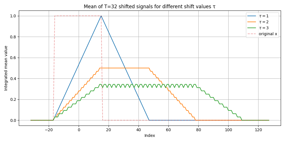
Note that the integrated image begins triangular for $\tau=1$, gradually becoming trapezoidal and wider for successive integer shift values $\tau \in [2, N]$, until we can imagine it ‘collapsing’ to a line for arbitrarily large N. Also recall from the previous blogpost that we briefly mentioned that $\operatorname{tri}(t) = \operatorname{rect}(t) \circledast \operatorname{rect}(t)$

Is this a coincidence? I think not! To better understand this, let’s express the integration operation in terms of a linear operation of the image with some kernel h. For a given shift $\tau$ the integration operation is equivalent to

Where $\star$ is the cross-correlation operation, and $h_{\tau}(x)= \sum_{t=0}^{N-1} \delta [x - t\tau]$ (note: this kernel is known as a Dirac comb).

Now for the case $\tau=1$ we have

which is another rectangular pulse! Finally then we get

Now that we understand how to think about 1D integration, let’s move on to more interesting things, mainly the phase-correlation algorithm, and surprising connection to our optimization objective.

Cross-correlation phase-transform (PHAT)

The phase-correlation algorithm is a well-known tool in signal processing for computing translation between two images, where it is based on the very simple notion of a phase transform.

Recall the duality

known as the Fourier shift-theorem.

Now if we have two signals $x_1, x_2$ where we know that $x_2[n] = x_1[n-n_0]$, we can solve for $n_0$ using what’s known as a phase transformation, which is an operation which extracts only the phase component of a Fourier-domain signal representation, equivalent to $e^{-j\omega n_0}$ in this case.

Let’s show this in action: using the Fourier shift theorem, we have

where $\overline{X_1}$ is the complex conjugate of $X_1$. Now the final step to compute $n_0$ is to take the inverse Fourier transform

Which results in a shifted Dirac delta (unit impulse) function. We note that the peak must appear at index $n_0$, meaning that we can solve for it by

where we only care about the real component of the resulting time-domain phase-transformed signal, meaning the component corresponding to the shifted Dirac delta.

Note that traditionally the $\mathop{\mathrm{arg\,max}}\limits_{n}$ operator is non-differentiable, in the sense that we scan $x_{PHAT}$ for an index yielding a maximum value.

What would be necessary then to make an equivalent differentiable implementation, yielding the same index? Could we formulate the algorithm as an optimization objective and solve for the correct shift via auto-differentiation?

Differentiable PHAT (‘naive’)

To get a better understanding of what’s happening in the final step of the algorithm, let’s explicitly write out the real part of $x_{PHAT}$:

Where $\Delta n = n - n_0$.

Is this a decent optimization objective? On the one hand we can be sure that by plugging in $n=n_0$ we obtain a global maxima, via

On the other hand, it is enough to confirm using centered frequency tiles $k’ = k - k_0, k_0=\frac{N-1}{2}$ that

Where $D_N$ is the Dirichlet kernel of order N. This can easily be factorized to

Where the right-hand form becomes highly oscillatory as N grows, meaning that this objective is insufficient for successful optimization.

Given what we’ve learned about the importance of bilinear interpolation as an effective low-pass filter in our original optimization objective, can we think of some ‘equivalent’ (dual) operation in the given case?

The Fejér kernel

The Fejér kernel is defined by

Meaning that the Nth Fejér kernel is built by integrating and smoothing the first N Dirichlet kernels. We can think of this operation as a ‘summation over summations’ (recall the definition of a Dirichlet kernel as a finite geometric series). Plugging in the explicit Dirichlet kernel formula (and skipping some math on the way) gives us the following explicit formula for a kernel of order N

meaning that the frequency representation of the Fejér kernel results in triangular weights, which we previously saw in the time-domain as a triangular kernel! Duality once again.

We understand then that the kernel is positive, and its corresponding frequency response is a steeper low-pass filter (less high-frequency components) than that of the Dirichlet kernel. This makes sense given our previously-gained knowledge that integration corresponds to low-pass filtering!

PHAT optimization objective (code)

Let’s show with some code that the Fejér kernel objective has better convergence properties than that of the Dirichlet kernel. Note that we use the frequency-domain representation of the kernel in our implementation.

import math
import torch
import matplotlib.pyplot as plt


def fejer_weights(C: torch.Tensor):
    """
    Fejér-type weights for a 1D spectrum C_alpha of shape (K,).
    Highest weight at DC (index 0), decaying linearly to ~0 at the highest index.
    """
    K = C.shape[0]
    device = C.device
    k = torch.arange(K, device=device)
    # normalized distance from DC [0..1]
    return 1.0 - k / (K - 1 + 1e-8)

def gcc_phat_objective(x1: torch.Tensor,
                              x2: torch.Tensor,
                              tau: torch.Tensor,
                              exclude_dc: bool = True,
                              method: str = "phat",
                             ) -> torch.Tensor:
    """
    f(tau) = Re{ mean_k [ C_normed[k] * exp(-i*ω_k*tau) ] }   (method="phat")
    or a Fejér-weighted surrogate (method="fejer").
    We maximize f(tau) over τ.
    """
    assert x1.shape == x2.shape and x1.ndim == 1
    
    M = x1.shape[0]
    k = torch.arange(M, dtype=x1.dtype, device=x1.device)
    omega = 2 * math.pi * k / M

    X1 = torch.fft.fft(x1)
    X2 = torch.fft.fft(x2)
    CPS = X1 * torch.conj(X2)
    mag = torch.clamp(torch.abs(CPS), min=1e-12)
    C_normed = CPS / mag     

    if exclude_dc:
        # ignore DC energy component
        C_normed = C_normed[1:]
        omega   = omega[1:]

    C_shifted = C_normed * torch.exp(-1j * omega * tau)  # minus → peak at true shift 
    if method == "fejer":
        # compute Fejer weights in frequency domain
        weights = fejer_weights(C_shifted)
        C_shifted *= weights
        
    dirichlet = torch.real(C_shifted)
    return dirichlet.mean()

# -----------------------------
# Inspect objective landscape
# -----------------------------
def plot_kernel_comparison(ax, taus_grid, x1, x2):
    """Plot Dirichlet vs Fejér kernel comparison on single axes with alpha=1, no interpolation"""
    dirichlet_vals = torch.tensor([float(gcc_phat_objective(x1, x2, t, method="dirichlet").detach())
                                   for t in taus_grid])
    ax.plot(taus_grid.numpy(), dirichlet_vals.numpy(), label='Dirichlet Kernel', linewidth=3)
    
    fejer_vals = torch.tensor([float(gcc_phat_objective(x1, x2, t, method="fejer").detach())
                                   for t in taus_grid])
    ax.plot(taus_grid.numpy(), fejer_vals.numpy(), label='Fejér Kernel', linewidth=3)
    
    # Add true shift line
    ax.axvline(0, linestyle="--", color='red', label="True Shift τ*", alpha=0.8, linewidth=2)
    
    ax.set_xlabel("Time Shift τ (samples)", fontsize=12)
    ax.set_ylabel("Objective Function f(τ)", fontsize=12)
    ax.set_title("Objective comparison", fontsize=14, fontweight='bold')
    ax.grid(True, alpha=0.3)
    ax.legend(fontsize=11)
    
# ground-truth shift of 0 for simple plotting
x_shifted=x
# Create plot
plt.figure(figsize=(14, 8))
ax = plt.gca()
taus_grid = torch.linspace(-6.0, 6.0, 201, dtype=torch.float64)  # Higher resolution
plot_kernel_comparison_single(ax, taus_grid, x1, x2)
plt.tight_layout()
plt.show()

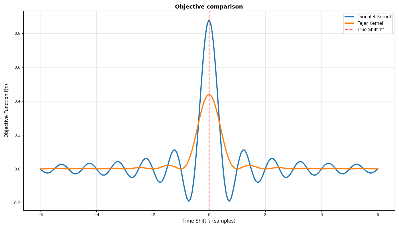
It becomes clear that although the Fejér kernel proves a better optimization objective than the Dirichlet, it is not a sufficient optimization objective in itself (what happens if we generate an initial shift which is arbitrarily far from the ground-truth shift?).

We fathom from this, that regardless of additional smoothing operations which can be applicable and yield better convergence, phase-information is most probably not sufficient in itself for establishing a feasible optimization objective.

Given this knowledge, how can we further improve our PHAT-based optimization objective?

Generalized Cross-Correlation (GCC)

The standard Generalized Cross-Correlation (GCC) function is defined in the frequency domain as:

where:

• $ G_{xy}(f) $ is the cross-power spectrum
• $ \Psi(f) $ is the spectral-weighting function

And the rest is simply the inverse Fourier Transform of the weighted cross-power spectrum.

Now what can we choose as our spectral-weighting function? To obtain our original phase-correlation algorithm it is sufficient to pass a zero-phase filter $ \Psi(f) = \frac{1}{|G_{xy}(f)|}$, which is the equivalent of normalizing the cross-power spectrum. However, we could choose any other filter $\Psi$ which suits our purpose.

A slight generalization of this idea which gives us a nice family of filters is to formulate $ \Psi(f) = 1/|G_{xy}(f)|^{\alpha}$, for $ \alpha \in [0, 1]$. For $ \alpha =1$ we get our original PHAT formulation, and for $ \alpha =0$ we have the original cross-power spectrum $G_{xy}$. We call this variant then GCC-PHAT, on account of its generating a whole “spectrum” (ha) between the phase-transformation and cross-power spectrum variants.

Let’s see the effect of varying this alpha on our optimization objective, slightly revising our previous code

def gcc_phat_objective(..., # all previous arguments
                              alpha=1, # new
                             ) -> torch.Tensor:
    ...     # as previously
    C_normed = CPS / (mag ** alpha)
    ...     # as previously
    

def plot_kernel_comparison(ax, taus_grid, x1, x2, alpha=1):
    """Plot Dirichlet vs Fejér kernel comparison on single axes with alpha=1, no interpolation"""
    dirichlet_vals = torch.tensor([float(gcc_phat_objective(x1, x2, t, method="dirichlet", alpha=alpha).detach())
                                   for t in taus_grid])
    ax.plot(taus_grid.numpy(), dirichlet_vals.numpy(), label='Dirichlet Kernel', linewidth=3)
    
    fejer_vals = torch.tensor([float(gcc_phat_objective(x1, x2, t, method="fejer", alpha=alpha).detach())
                                   for t in taus_grid])
    ... # as previously

# Create plot
plt.figure(figsize=(14, 8))
ax = plt.gca()
taus_grid = torch.linspace(-6.0, 6.0, 201, dtype=torch.float64)  # Higher resolution
plot_kernel_comparison(ax, taus_grid, x1, x2, alpha=0.7)
plt.tight_layout()
plt.show()

Now the Fejér-smoothed objective is starting to look like decent! A randomly-initialized shift value has some guarantee of converging to the correct ground-truth shift with a ‘smart’-enough optimizer. Can we intuitively understand why this is the case?

There are additional improvements which can be made to reduce some swells (high-frequency components) in the optimization landscape. For example- what would be the effect of integrating the Fejér kernels as we previously did to the Dirichlets (Hint- integration is a smoothing operation, and thus a low-pass filter)?

GCC-PHAT for noisy signal sequences

Suppose that we are working with a video consisting of noisy frames, where the noise is static (we will see later what and how this has to do with occlusion). This means that we model each noisy frame as $I_t = W^t(I_0, \tau^*) + V$, with V representing the constant noise mask. Now, we want to estimate a cohesive-translation motion model (same translation between each pair of frames) over this video.

A naive approach would be to compute phase-correlation between a given pair of images. Note that for any such pair some variant of GCC-PHAT would yield a translation of $\tau=0$ (why?). Instead, we can use our knowledge from this previous blogpost regarding the moving-average filter (specifically that it is optimal for denoising) to integrate our video into a pair of integrated images, and then use a variant of GCC-PHAT over this pair!

We obtain a pair of integrated images by partitioning our video into even and odd frame subsets, and then compute integrated images in the following way:

where $\phi = \frac{\tau}{W}, \quad \Delta \phi = \frac{\tau - \tau^*}{W}$ and $ \mathcal{H_{\frac{N}{2}}}(\phi)$ is a moving-average filter of order $\frac{N}{2}$ (see previous blog-post) with frequency responses parameterized by $\phi$.

$I_{odd}$ is constructed similarly over frames with odd time-steps, with the only exception

Meaning that all odd-frames are mapped translated back to the reference odd frame (why we do it this way will become clear soon).

Note that of the two moving-average filters derived in the equation, $\mathcal{H_{\frac{N}{2}}}(\Delta \phi)$ depends on the ground-truth shift, while $\mathcal{H_{\frac{N}{2}}}(\phi)$ doesn’t, meaning that noise reduction is independent of the ground-truth shift. On the other hand, for ‘zero-motion’ ($\tau=0$) noise energy is maximised, which creates a spurious (false) maxima in our optimization problem. This is the reason why computing phase correlation between any pair of noisy images doesn’t work in this case!

Now coming back to our integrated images, note that

From here computing GCC-PHAT is straightforward, where we have

Let’s plug in different values for $\alpha$! Starting with $\alpha=0$ we get

Note that optimizing over the magnitude of this signal

is equivalent to our original optimization objective, up to the order of the moving average filter!

Now as N grows we have

Using the fact that the moving-average filter reduces noise by approximately the square-root of its order (see explanation elsewhere), meaning that the effect of the noise-component becomes negligable compared to that of the signal.

Connecting the two optimization objectives

Finally, note that we can “revert” our GCC-PHAT objective into the exact previous objective by computing the integrated image from integrated pairs by

We’ve essentially created a link between our two optimization objectives, where we can choose either depending on our need for flexibility, computational constraints.

Conclusion

We now have “pure” energy (magnitude) and phase “flavors” of our GCC-PHAT objective, obtainable by choosing spectral-weighting factors $\alpha\in\lbrace {0,1} \rbrace$ respectively, where we’ve seen that $\alpha=0$ gives us our previous variance optimization objective, and $\alpha=1$ the PHAT optimization objective (up to necessary interpolation/smoothing operations). Comparing these two objectives, the variance objective maximizes coherent energy, where an incorrect shift creates destructive interference. On the other hand, for the PHAT objective the phase component is used to align a sharp correlation peak, which is smoothed by the Fejér kernel.

We can treat the first as a more “global” method, while the second is more “local”. The need for a trade-off between these two comes up in the case of noisy signals, in which the additive nature of the Fourier transform causes both phase and magnitude information to be offset/randomized by the noisy component. It makes sense then in this case to utilize a mix of both when computing the ground truth shift.

We’ll make a comparison of the utility of these different objectives in the next blogpost, using samples of clean and noisy image pairs.

Until then!

Tweet Share