Motion Under Occlusion, pt.3: Bilinear Interpolation as a Filter

This post continues from pt.2, where we showed that the Fourier-domain implementation of our objective is ~2.5× faster. Now we look at why naive Fourier optimization fails, and how bilinear interpolation fixes it.

Fourier-domain optimization (continued)

Just to remind, our Fourier-domain objective formulation is:

where

Where $\mathcal{H_T}(\Delta \phi)$ is known as a moving-average filter of order T. We will learn more about the nature of this filter in this current blog-post, as well as why it is insufficient in itself for successful Fourier-domain optimization.

First optimization trial (naive)

In order to compute the motion of an input video, we need to slightly tweak our Fourier-objective (recall that it is a function of the displacement $\Delta\phi$, which we do not know at the time of computation, as it depends on the ground-truth shift $\theta*$) We must take this into account then in our code-implementation, more specifically, instead of computing the analytical closed-form geometric sum, we need to explicitly compute the sum from the input frames. We obtain then the following implementation

def fourier_pipeline_video(frames: torch.Tensor, shifts: torch.Tensor,
                           fourier_input=False):
    """
    Fully differentiable Fourier-domain warping and integration.
    Args:
        frames: (B, T, H, W) spatial frames
        shifts: (B, 2) shift vector per batch
    Returns:
        integrated_fft: (B, H, W) integrated FFT
        variance_fft: (B,) variance-like scalar
    """
    B, T, H, W = frames.shape

    if not fourier_input:
        X = torch.fft.fft2(frames, norm='forward', dim=(-2, -1))
    else:
        X = frames

    v, u = torch.meshgrid(
        torch.arange(H, device=frames.device, dtype=X.real.dtype),
        torch.arange(W, device=frames.device, dtype=X.real.dtype),
        indexing='ij'
    )

    shifts_exp = shifts.view(B, 1, 1, 2)
    omega = (u.unsqueeze(0) * shifts_exp[..., 0] / W
             + v.unsqueeze(0) * shifts_exp[..., 1] / H)  # (B,H,W)
    omega = omega.unsqueeze(1)  # (B,1,H,W)

    base_phase = torch.exp(-2j * torch.pi * omega)
    t = torch.arange(T, device=frames.device, dtype=X.real.dtype).view(1, T, 1, 1)
    phase_shifts = (base_phase * (1 - base_alpha)) ** t if weighted else base_phase ** t

    shifted = X * phase_shifts  # (B,T,H,W)
    integrated_fft = shifted.sum(dim=1) / T

    mag2 = integrated_fft.real ** 2 + integrated_fft.imag ** 2
    dc_power = mag2[..., 0, 0]
    variance_fft = mag2.sum(dim=(-2, -1)) - dc_power

    return integrated_fft, variance_fft

Note that the spatial pipeline can already deal with video input (see pt.1). The following code runs the optimization in both domains and compares results:

import itertools

# estimated shifts should be within this distance from GT for successful optimization   
SUCCESS_CRIT = 1/T

# Wrappers for evaluating functions
fourier_wrapper = lambda videos, shifts, weighted: fourier_pipeline_video(videos, shifts, weighted=weighted, fourier_input=True, interpolate=True) 
spatial_wrapper = lambda videos, shifts, weighted: spatial_pipeline(videos, videos.shape[1], shifts, weighted=weighted)

def compute_motion(eval_fn, videos, max_steps=400, thresh=SUCCESS_CRIT, num_trials=T, verbose=False):
    """
    Compute motion via optimization over videos using eval_fn (spatial/fourier pipeline).
    """
    def initialize_shifts(n_trial):
        torch.manual_seed(n_trial)
        init_shifts = (torch.rand(2*B).reshape(B,2) * 2 - 1) * (B*SHIFT_SCALE)  
        return init_shifts.clone().detach().requires_grad_(True)

    all_trials_results = []

    for trial in range(num_trials):
        shifts = initialize_shifts(trial)
        optimizer = torch.optim.Adam([shifts], lr=0.5)
        scheduler = torch.optim.lr_scheduler.ReduceLROnPlateau(optimizer, mode='min', patience=50, factor=0.5)

        all_shifts = []
        deviations = []
        converged = False

        for step in range(max_steps):
            optimizer.zero_grad()
            _, _, var_batches = fourier_wrapper(videos, shifts) if eval_fn == "fourier" \
                                else spatial_wrapper(videos, shifts)
            loss = -var_batches.mean()
            loss.backward()
            optimizer.step()
            scheduler.step(loss)

            current_shifts = shifts.detach().clone()
            deviation = torch.norm(current_shifts - GT_SHIFTS).item()
            all_shifts.append(current_shifts)
            deviations.append(deviation)

            if deviation < thresh and step > 100:
                converged = True
                break

        all_trials_results.append({
            'final_shifts': all_shifts[-1],
            'final_deviation': deviations[-1],
            'converged': converged,
            'steps': step + 1,
            'all_shifts': all_shifts,
            'deviations': deviations
        })

    num_converged = sum(1 for r in all_trials_results if r['converged'])
    if verbose: print(f"Total successful convergences: {num_converged}/{num_trials}")

    return all_trials_results, num_converged


def compare_configs(configurations, inputs, num_trials=10, verbose=True, **kwargs):
    """
    Evaluate motion computation for each pipeline configuration.
    """
    comparison_results = {}
    success_counts = {}
    input_spatial, input_fourier = inputs

    if verbose: 
        print(f"GT shifts: {GT_SHIFTS}") 

    for config in configurations:
        eval_fn = config
        videos = input_spatial.clone().detach().requires_grad_(True) if eval_fn=="spatial" else \
                input_fourier.clone().detach().requires_grad_(True)
        config_name = f"{eval_fn}"
        if verbose: print(f"\n=== Running {config_name} pipeline ===")
        results, num_converged = compute_motion(
                eval_fn=eval_fn,
                videos=videos,
                num_trials=num_trials,
                verbose=verbose,
                **kwargs
            )
        comparison_results[config_name] = results
        success_counts[config_name] = num_converged

    if verbose:
        print("\n=== Convergence Summary ===")
        for config_name, num_converged in success_counts.items():
            print(f"{config_name}: {num_converged}/{num_trials} successful convergences")

    return comparison_results, success_counts

methods = ["spatial", "fourier"]
results, _ = compare_configs(methods, (input_spatial, input_fourier))

We run this code, obtaining the following

GT shifts: tensor([[ 4,  2],
    [ 0, -2]])

=== Running spatial pipeline ===
Total successful convergences: 10/10

=== Running fourier pipeline ===
Total successful convergences: 0/10

Let’s plot the loss landscapes to see why:

# Plot loss contour and optimization path
N = 20           # number of initial steps to plot
batch_idx = 0    # batch to visualize
shift_range = 2*B*SHIFT_SCALE
mesh_resolution = shift_range**2  # number of points per axis

# Grid for contour
x = torch.linspace(-shift_range, shift_range, mesh_resolution)
y = torch.linspace(-shift_range, shift_range, mesh_resolution)
X_grid, Y_grid = torch.meshgrid(x, y, indexing='ij')

# Prepare figure
fig, axes = plt.subplots(len(configurations)//2, 2, figsize=(14, 12))
axes = axes.flatten()

for idx, (method, weighted) in enumerate(configurations):
    loss_grid = torch.zeros_like(X_grid)

    if method == "spatial":
        frames_plot = input_spatial.clone().detach().requires_grad_(False)
        pipeline_fn = spatial_pipeline
    else:
        frames_plot = input_fourier.clone().detach().requires_grad_(False)
        pipeline_fn = lambda f, T, s: fourier_pipeline_video(f, s, fourier_input=True)

    for i in range(mesh_resolution):
        for j in range(mesh_resolution):
            test_shift = torch.zeros(B, 2)
            test_shift[batch_idx, 0] = X_grid[i,j]
            test_shift[batch_idx, 1] = Y_grid[i,j]
            _, _, var_batch = pipeline_fn(frames_plot, frames_plot.shape[1] if method=="spatial" else T, test_shift)
            loss_grid[i,j] = var_batch[batch_idx].item()

    X_np, Y_np, Z_np = X_grid.numpy(), Y_grid.numpy(), loss_grid.numpy()
    ax = axes[idx]
    contour = ax.contourf(X_np, Y_np, Z_np, levels=50, cmap='viridis')
    fig.colorbar(contour, ax=ax)
    ax.set_title(f"{method.capitalize()}")
    ax.set_xlabel('Shift dx')
    ax.set_ylabel('Shift dy')

    trial_result = results[f"{method}"][0]
    shifts_for_plot = trial_result['all_shifts'][:N]
    shifts_np = torch.stack(shifts_for_plot).numpy()[:, batch_idx, :]
    ax.plot(shifts_np[:,0], shifts_np[:,1], 'r-o', label='Optimization steps')
    ax.scatter(GT_SHIFTS[batch_idx,0], GT_SHIFTS[batch_idx,1], color='red', marker='x', s=60, label='GT')
    ax.legend()

plt.tight_layout()
plt.show()

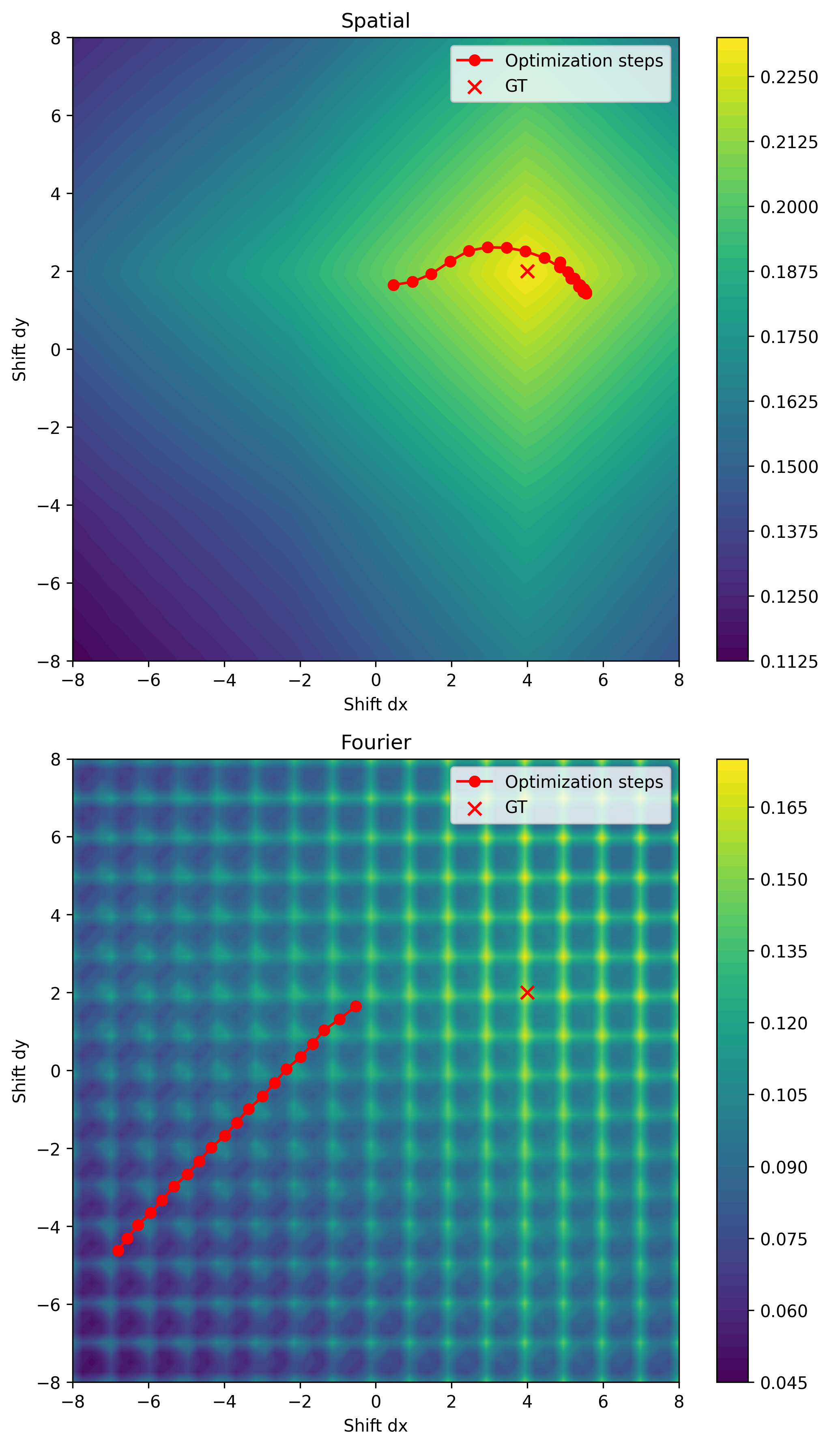
Hmm, the loss landscapes do not look the same at all. While the spatial domain implementation results in a smooth landscape, in the Fourier-domain we get a certain “grid”-ness which is a bit hard to make sense of. More specifically we have periodic local maxima (at integer-valued shifts), which disrupt optimization. In order to better understand this phenomenon let’s analyse the behavior of the previously-mentioned moving-average filter, and see what it has to do with it.

Moving average filter- frequency response

We begin by finding an analytical representation for the moving average filter frequency response, via

Note that we have separated the moving-average filter into phase and magnitude components, meaning that computing the frequency response from here is straightforward. The magnitude usually ends up looking something like (found this online, forgive the spelling mistake in the title)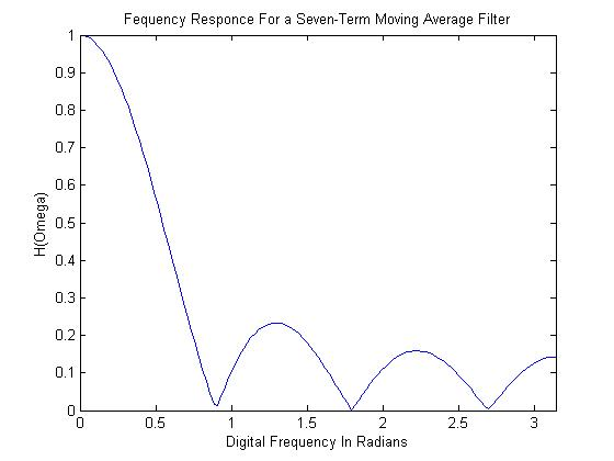

Where in this case we see the magnitude spectrum of a 7-tap ($T=7$) moving-average filter. We see that the filter generally has a low-pass behavior, with certain ‘richochets’ or rebounds of magnitude, which we will see later lead to all kinds of problems.

Let’s get some perspective on the filter from an experienced practitioner, via The Scientist and Engineer’s Guide to Digital Signal Processing:

Not only is the moving average filter very good for many applications, it is optimal for a common problem, reducing random white noise while keeping the sharpest step response. Of all the possible linear filters that could be used, the moving average produces the lowest noise for a given edge sharpness. The amount of noise reduction is equal to the square-root of the number of points in the average.

On the one hand then, this is the “filter for the job”, in the sense that once we begin to deal with occlusion, we will want to choose a filter which gets rid of noise (occlusion) optimally for our optimization purposes.

One the other hand, just a few pages later we get the following

The roll-off is very slow and the stopband attenuation is ghastly. Clearly, the moving average filter cannot separate one band of frequencies from another. In short, the moving average is an exceptionally good smoothing filter (the action in the time domain), but an exceptionally bad low-pass filter (the action in the frequency domain).

Now then, looking back to the loss landscape for the Fourier optimization objective, we perceive a general trend of increase in variance (signal energy) when approaching the ground truth shift, but an additional side-effect is a radial-oscillation pattern prevalent around integer-valued shifts, where energy seems to spike. This phenomenon is a type of spectral-leakage.

Given our newly-gained knowledge about the behavior of the moving-average filter and its less-than-sufficient attenuation, we can interpret this oscillation as an artifact caused by the “left-over” high-frequency components after filtering. In other words, we need additional attenuation of high-frequency content in the integrated image for optimization to work, meaning that additional low-pass filtering is necessary.

Bilinear interpolation as a low-pass filter

Going back to the difference between spatial and Fourier domains, we note that the one operation which we didn’t previously address was bilinear interpolation in the frame warping. The initial motivation for this operation was to ensure differentiability for the spatial-domain optimization (recall that “rolling” the image frames is non-differentiable), where “bilinear interpolation is arguably the simplest possible separable method that produces a con- tinuous (differentiable) function”¹. Consequently, the operation has profound consequences in the Fourier domain as well.

Let’s get to know these by modelling the operator first as a kernel in the time/spatial domain, and then looking at its Fourier-equivalent operator.

The linear interpolation kernel (also called the triangular kernel) is defined as

For bilinear interpolation in two dimensions, we use the separable extension of this kernel. If $k(t)$ is the 1-D interpolation kernel, then the 2-D bilinear interpolation kernel is

This means that bilinear interpolation is performed by convolving the signal/image first along one axis using k, and then along the other axis using the same kernel.

The triangular kernel can be written as the convolution of two rectangular functions:

This proves useful for computing the Fourier transform of the kernel, where using the dualities $\circledast \;\overset{\text{FT}}{\longleftrightarrow}\; \times , \operatorname{rect} \overset{\text{FT}}{\longleftrightarrow} \operatorname{sinc}$ (see this blogpost) we get:

Meaning the bilinear interpolation kernel is equivalent to a squared sinc function in the frequency domain. What is the interpretation of the frequency response of this filter? Obviously it is quite close in nature to the squared frequency response of the moving average filter, but whereas the latter is periodic, sinc decays over time. We can easily show that the former has better high-frequency suppression, via the inequality

Where the last two expressions are the squared moving average filter and bilinear interpolation frequency responses respectively. It makes sense then to apply both of these operations to obtain a smoother, more convex optimization landscape. We can exhibit this behavior by looking at the frequency responses of each of the filters, as well as a cascade (product in the frequency-domain) of the two: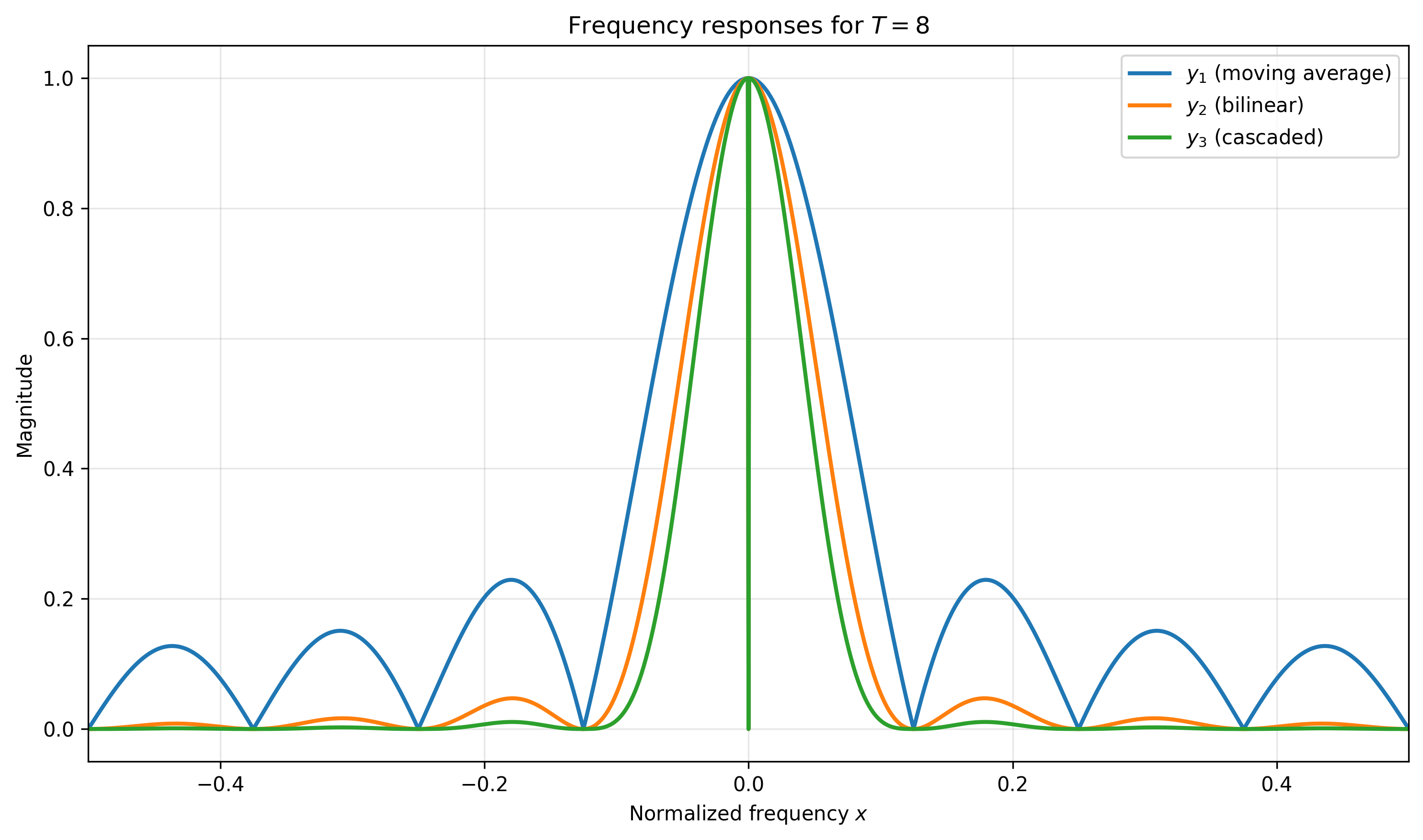

Note that the cascaded filters frequency response (green) has virtually no magnitude for frequency beyond the stop-band frequency of $\frac{1}{T}=0.125$, meaning our optimization landscape should now be in much better shape!

Second optimization trial (with interpolation)

We implement the frequency-domain interpolation in code as follows:

def make_sinc_2d(u, v, W, H):
    # Separate u and v components for proper 2D bilinear
    u_norm = u.unsqueeze(0) / W  # Normalized frequencies
    v_norm = v.unsqueeze(0) / H
    
    # 2D separable bilinear kernel
    sinc_u = torch.sinc(u_norm) ** 2  # Smooth in u-direction
    sinc_v = torch.sinc(v_norm) ** 2  # Smooth in v-direction  
    sinc_2d = sinc_u * sinc_v
    return sinc_2d

And incorporate it into our own existing code

def fourier_pipeline_video(frames: torch.Tensor, shifts: torch.Tensor,
                           weighted=False, fourier_input=False, base_alpha=BASE_ALPHA,
                           interpolate=False):
    """
    Fully differentiable Fourier-domain warping and integration.
    Args:
        frames: (B, T, H, W) spatial frames
        shifts: (B, 2) shift vector per batch
        interpolate: whether to apply bilinear interpolation
    Returns:
        shifted: (B, T, H, W) phase-shifted FFTs
        integrated_fft: (B, H, W) integrated FFT
        total_power: (B,) variance-like scalar
    """
    # ... (no change to previous code)
    if interpolate:
        sinc_2d = make_sinc_2d(u, v, W, H)
        shifted = X * phase_shifts * sinc_2d.unsqueeze(1)
    else:
        shifted = X * phase_shifts

    # ... (no change to next code)
    return shifted, integrated_fft, total_power

We are now ready to run our code once more, obtaining the following optimization results

GT shifts: tensor([[ 4,  2],
    [ 0, -2]])

=== Running spatial pipeline ===
Total successful convergences: 10/10

=== Running fourier pipeline ===
Total successful convergences: 10/10

and the following loss landscape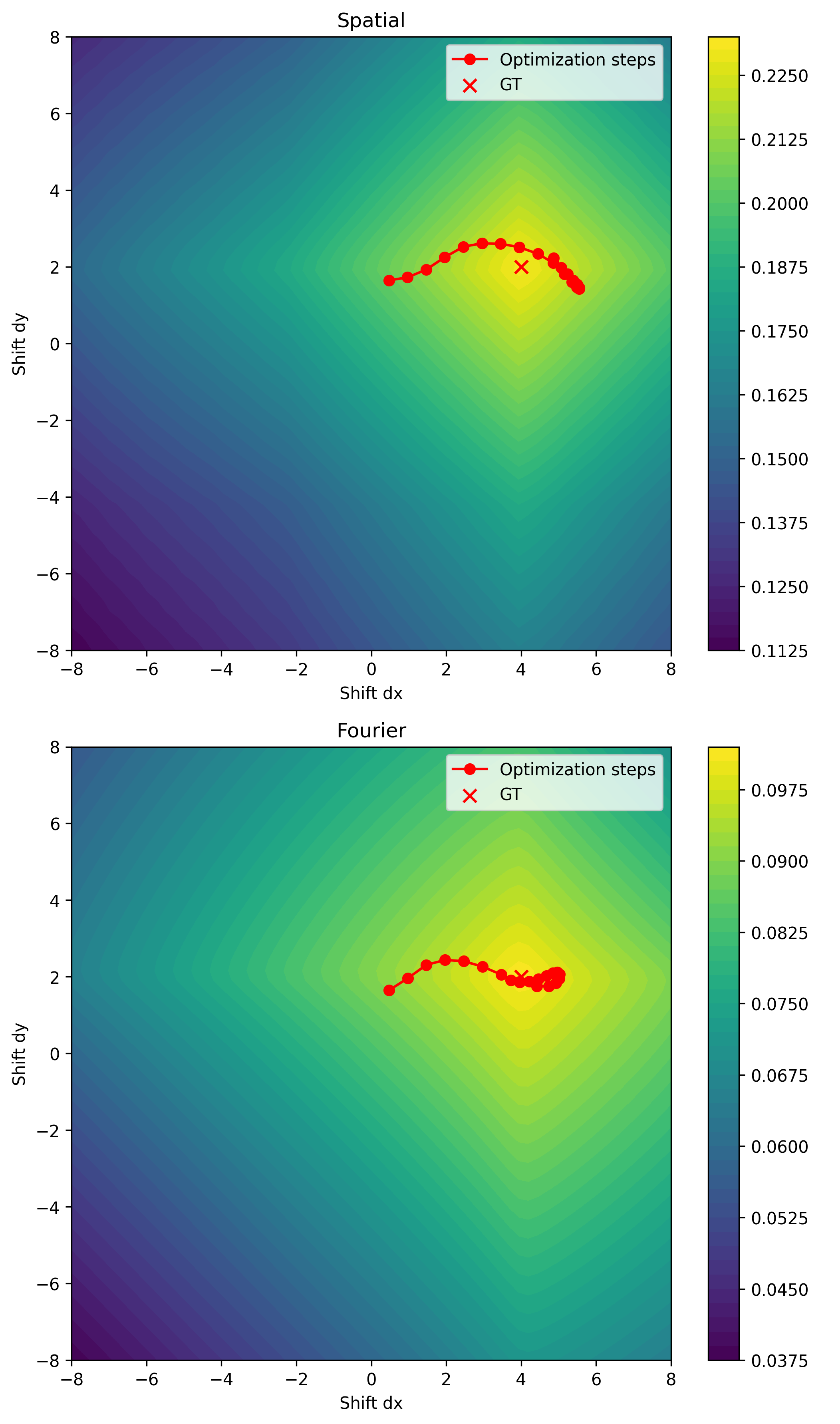

Success! Note also that the shift estimates in the Fourier domain appear to converge slightly faster (end up generally closer) to the ground truth shift than in the spatial-domain case.

Conclusion

We’ve discovered that not only is bilinear interpolation sufficient for optimization (by providing differentiability in the spatial domain implementation), but it is also necessary for ensuring that our optimization landscape is smooth and convex.

Note however that in our Fourier domain implementation we are not bound to use interpolation (as in the spatial domain case, where it is very efficient to compute), but rather may choose any suitable low-pass filters. There are better possibilities out there, such as the Lanczos filter, which may pop back in the next blog-posts! Stay tuned.

Next time, we’ll take a look at some of the more theoretical aspects of the problem, mostly through the connection of our optimization objective to a well-known signal processing algorithm known as generalized cross-correlation phase transform (GCC-PHAT). We will go down to 1D for more simplified analytical forms, which will once more give us additional intuition. Most importantly, we will begin discussing possible models for occlusion, and see how these affect our notion of the problem, objective, etc…

See you next time!

Tweet Share