Moving from 4→6DoF motion computation via anisotropic scale refinement
- 4 minsIntroduction
Most classical image registration pipelines assume a 4-degree-of-freedom motion model: translation, rotation, and isotropic scale. While sufficient in many situations, real-world deformations frequently include anisotropic scaling or shear, which together require a full 6-DoF affine model.
This post explores a simple idea: keep the efficiency of Fourier–Mellin (FM) for similarity alignment, and add a lightweight refinement step that estimates the remaining anisotropic stretch.
Part A — Method
The linear component
Let a reference image $I_{\mathrm{ref}}$ and moving image $I_{\mathrm{mov}}$ be related by
\[x \mapsto A x,\qquad A\in \mathrm{GL}(2).\]Translation can be handled separately via phase correlation, so we focus on the linear component $A$.
Polar decomposition
Using the polar decomposition,
\[A = R\,P, \quad R\in \mathrm{SO}(2),\quad P\succ 0\]where
- $R$ represents rotation
- $P$ is a symmetric positive-definite stretch matrix
The stretch admits the eigen-decomposition
\[P = Q\,\mathrm{diag}(\lambda_1,\lambda_2)\,Q^\top\]with $\lambda_1\ge \lambda_2>0$.
The anisotropy is captured by the condition number
\[\kappa = \frac{\lambda_1}{\lambda_2}.\]Isotropic–anisotropic parameterization
We factor the stretch as
\[P = \lambda_{\mathrm{iso}}\,S_{\mathrm{ani}}(\delta,\phi)\]with
\[S_{\mathrm{ani}}(\delta,\phi) = R(\phi)\,\mathrm{diag}(e^\delta,e^{-\delta})\,R(-\phi).\]Matching eigenvalues gives
\[\lambda_1 = \lambda_{\mathrm{iso}} e^\delta,\qquad \lambda_2 = \lambda_{\mathrm{iso}} e^{-\delta}.\]From this,
\[\lambda_{\mathrm{iso}} = \sqrt{\lambda_1\lambda_2}, \qquad \delta = \tfrac12\log\frac{\lambda_1}{\lambda_2}.\]Thus isotropic stretch corresponds to $\delta=0$.
Baseline: Fourier–Mellin
The classical FM pipeline estimates similarity transforms:
- Compute Fourier magnitude (removes translation).
- Map to log-polar coordinates.
- Use phase correlation to recover rotation and isotropic scale.
After applying the similarity correction we obtain $I_{\mathrm{cur}}$, which may still contain anisotropic stretch.
Log-polar view of anisotropy
Let $u(\alpha)=(\cos\alpha,\sin\alpha)$.
The anisotropic stretch scales direction $\alpha$ by
\[g(\alpha)=\|S_{\mathrm{ani}}(\delta,\phi)u(\alpha)\|.\]This yields
\[g^2(\alpha)= e^{2\delta}\cos^2(\alpha-\phi)+ e^{-2\delta}\sin^2(\alpha-\phi).\]In log-polar coordinates a radial scale becomes an additive shift:
\[\rho=\log r \mapsto \rho+\log g.\]Thus the anisotropic distortion produces an angle-dependent radial shift
\[s(\alpha)=\log g(\alpha).\]Small-anisotropy approximation
For small $|\delta|$,
\[e^{\pm2\delta}\approx 1\pm2\delta.\]Substituting into $g(\alpha)$ gives
\[s(\alpha)\approx \delta\cos(2(\alpha-\phi)).\]So anisotropy appears as a second harmonic sinusoid in the log-polar shift curve.
Estimating the shift curve
Working in the log-polar Fourier magnitude
\[M(\alpha,\rho)=\mathcal{L}(|\mathcal{F}(I)|)\]the anisotropic distortion produces
\[M_{\mathrm{cur}}(\alpha,\rho) \approx M_{\mathrm{ref}}(\alpha,\rho-s(\alpha)).\]For each angular bin we estimate the radial shift using 1-D phase correlation, producing samples
\[\hat{\mathbf{s}} = [\hat s_0,\ldots,\hat s_{H_\alpha-1}].\]Recovering anisotropy
We fit the second harmonic
\[\hat s(\alpha) = a_0+a_c\cos(2\alpha)+a_s\sin(2\alpha).\]This corresponds to
\[A=\sqrt{a_c^2+a_s^2}, \qquad \phi=\tfrac12\operatorname{atan2}(a_s,a_c).\]The anisotropy parameter follows as
\[\delta \approx A\log(b)\]where $b$ is the log-polar radial base.
Refinement loop
The full algorithm alternates between similarity removal and anisotropy estimation:
-
FM step
Estimate isotropic scale and rotation. -
Anisotropy estimation
Measure per-angle radial shifts and fit the harmonic model. -
Resolve discrete ambiguities
Evaluate candidates
$(\pm\delta,\phi)$ and $(\pm\delta,\phi+\pi/2)$
and select the best alignment score. -
Accumulate and iterate
Only a few outer iterations are required.
Part B — Experiment
We evaluate the approach on 5,000 affNIST image pairs, where ground-truth affine parameters are available.
Quantitative summary
The table below compares the recovered singular values with/out anisotropic refinement (2 steps).
| Metric | Baseline (FM) | Refined ($\delta, \phi$) | Change |
|---|---|---|---|
| MAE($\lambda_1$) | 0.094 | 0.077 | −18.1% |
| MAE($\lambda_2$) | 0.092 | 0.063 | −31.5% |
| RMSE($\lambda_1$) | 0.121 | 0.111 | −8.3% |
| RMSE($\lambda_2$) | 0.117 | 0.090 | −23.1% |
The refinement consistently improves recovery of both singular values, with the largest gains for the smaller eigenvalue $\lambda_2$.
The anisotropy estimate itself remains the most challenging part of the problem. The recovered parameter $\delta$ reaches $\sim 0.3$ correlation with ground truth, and tends to underestimate deformation magnitude:
\[\mathbb{E}[\hat{\delta}] = 0.04 \qquad \mathbb{E}[\delta_{\mathrm{gt}}] = 0.09.\]This indicates that while the refinement steps improve the recovered affine scales, the magnitude of anisotropy is still systematically under-estimated.
Parameter distributions
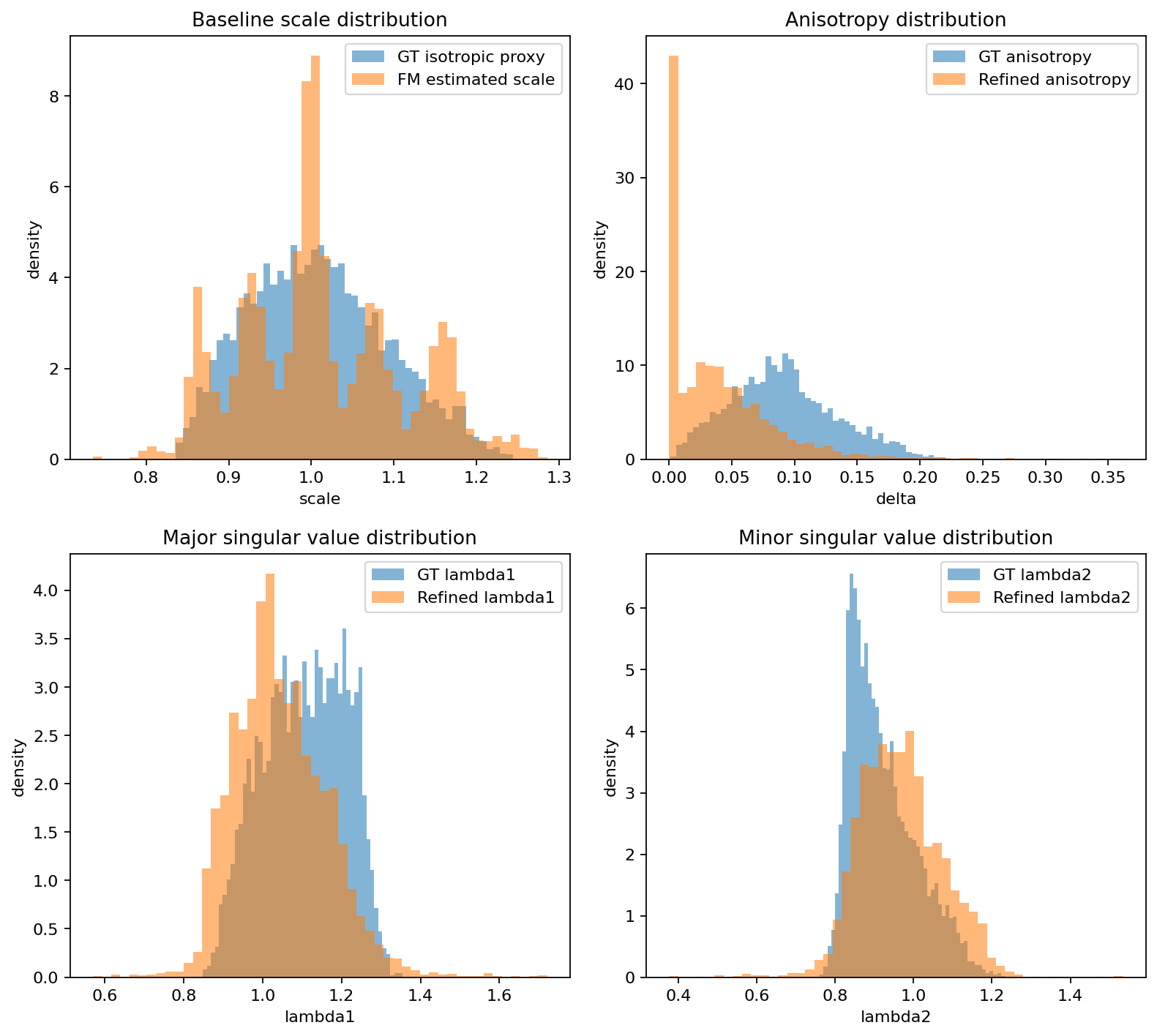 The isotropic scale estimates exhibit mild quantization. Because Fourier–Mellin measures scale as a translation along the discretized log-radius axis, each bin corresponds to a fixed multiplicative scale step. This produces slight clustering in the recovered scale distribution.
The anisotropic estimates exhibit prominent bias toward smaller values, which cause the recovered singular values to cluster near the isotropic scale.
Final thoughts
This experiment shows that classical Fourier–Mellin registration can be extended toward affine alignment using a lightweight anisotropic refinement.
While anisotropy estimation remains noisy and tends to underestimate deformation magnitude, the refinement consistently improves recovered affine scales.
In practice the method works well as:
- a fast initialization for full affine registration, or
- a cheap refinement layer on top of similarity alignment.
More broadly, it highlights how far classical frequency-domain techniques can be pushed with careful modeling and a modest amount of engineering.