Motion Under Occlusion, pt.5: The Occlusion Bias
- 5 minspt.4 derived the GCC-PHAT objective for clean video. This post adds a static noise component, traces how it creates a spurious zero-motion maximum, extends the same argument to 2D static occlusion, and then asks empirically: does working in the Fourier domain help?
The zero-motion bias
Suppose each frame contains a static noise mask $V$:
\(I_t = W^t(I_0,\,\tau^*) + V.\)
We follow the same even/odd split from pt.4. Integrating over even-indexed frames and applying the shift theorem gives
\(I_{even} = \mathcal{H}_{\frac{T}{2}}(\Delta\phi) \cdot \mathcal{F} \lbrace I_0 \rbrace + \mathcal{H}_{\frac{T}{2}}(\phi) \cdot \mathcal{F} \lbrace V \rbrace\)
where $\phi = \tau/M$, $\Delta\phi = (\tau - \tau^*)/M$, and $\mathcal{H}_{T/2}$ is the moving-average filter of order $T/2$ from pt.3. The first term is maximized at the true shift ($\Delta\phi = 0$); the second depends only on $\phi$ and peaks at zero motion ($\phi = 0$).
The bias arises at $\tau = 0$: there $\phi = 0$ and $\mathcal{H}_{T/2}(0) = 1$, so the noise term reaches its maximum. Any method that measures image similarity on raw frames — including plain phase correlation — sees a spurious peak at zero motion.
Since $I_{odd} = e^{-j\omega\phi^*} \cdot I_{even}$ (derived in pt.4), the GCC-PHAT cross-spectrum simplifies to
\(\frac{I_{odd} \cdot \overline{I_{even}}}{|I_{odd} \cdot \overline{I_{even}}|^\alpha} = |I_{even}|^{2(1-\alpha)} e^{-j\omega\phi^*}\)
Setting $\alpha = 0.5$ and using the fact that the moving-average filter attenuates noise energy by $\sqrt{T/2}$,
\(|I_{even}| \cdot e^{-j\omega\phi^*} \approx |\mathcal{H}_{\frac{T}{2}}(\Delta\phi) \cdot \mathcal{F} \lbrace I_0 \rbrace + \frac{\mathcal{F} \lbrace V \rbrace}{\sqrt{T/2}}| \cdot e^{-j\omega\phi^*}\)
As $N \to \infty$ the noise term vanishes and we recover the clean signal:
\(\begin{aligned} \lim_{T \to \infty} |\mathcal{H}_{\frac{T}{2}}(\Delta\phi) \cdot \mathcal{F} \lbrace I_0 \rbrace + \frac{\mathcal{F} \lbrace V \rbrace}{\sqrt{T/2}}| \cdot e^{-j\omega\phi^*} \\[4pt] &= |\mathcal{H}_{\infty}(\Delta\phi) \cdot \mathcal{F} \lbrace I_0 \rbrace| \cdot e^{-j\omega\phi^*} \end{aligned}\)
For finite $T$ the bias persists, but GCC-PHAT with $\alpha = 0.5$ suppresses it: the spectral whitening down-weights bins dominated by $V$, and as $T$ grows the noise term shrinks as $1/\sqrt{T/2}$.
2D case
For static 2D occlusion the structure is identical, but this large-$T$ fix no longer applies. Model each frame as a moving target with a static occluder layered on top:
\(I_t = W^t(I_{\mathrm{mov}},\,\theta^*) + I_{\mathrm{occ}}.\)
For an example of such a video in the 2DoF case:
By the shift theorem and linearity, the integrated image becomes
\(\mathcal{F} \lbrace \overline{I}(\theta) \rbrace = H(\Delta\phi) \cdot \mathcal{F} \lbrace I_{\mathrm{mov}} \rbrace + H(\phi) \cdot \mathcal{F} \lbrace I_{\mathrm{occ}} \rbrace\)
where $H$ is the moving-average filter from pt.2, and the variance objective becomes
\(f_{\mathrm{opt}}(\theta) \overset{\text{DFT}}{\leftrightarrow} \sum_{(m,n)\neq(0,0)} |H(\Delta\phi) \cdot \mathcal{F} \lbrace I_{\mathrm{mov}} \rbrace + H(\phi) \cdot \mathcal{F} \lbrace I_{\mathrm{occ}} \rbrace|^2\)
The first term is maximized at the true motion $\theta^*$; the second at zero motion. Unlike $\mathcal{F}\lbrace V \rbrace / \sqrt{T/2}$, the occluder term $H(\phi) \cdot \mathcal{F} \lbrace I_{\mathrm{occ}} \rbrace$ does not shrink with $T$ — integrating more frames cannot wash out a fixed-energy occluder. At high occlusion density the zero-motion term wins regardless of domain.
This asymmetry also shapes the choice of objective for the experiment below. GCC-PHAT’s advantage over the plain variance objective requires many frames to activate (the $1/\sqrt{T/2}$ factor needs large $T$). With $T = 8$ frames that advantage hasn’t kicked in, so both methods below use the variance objective — making the comparison a clean test of domain (spatial vs. Fourier), not algorithm.
Experiment: spatial vs. Fourier domain motion estimation
We’ve shown that occlusion injects a bias no amount of integration can remove. But theory says nothing about magnitude: how quickly does increasing occlusion density hurt convergence, and does the Fourier domain formulation offer any practical advantage in the regime where both methods are expected to struggle? To answer this we run a controlled experiment on synthetic video under varying occlusion density.
Metric. Motion estimation quality is measured by end-point error (EPE) — the Euclidean distance in pixels between the estimated shift $\hat\tau$ and the ground truth $\tau^*$:
\(\mathrm{EPE} = \|\hat\tau - \tau^*\|_2\)
EPE is the standard evaluation metric in optical flow, where sub-half-pixel accuracy is the target. A trial counts as successful if EPE < 0.5 after optimization. We also track time-to-threshold (TTT): the median number of optimizer steps to first achieve EPE < 0.5 — a measure of convergence speed rather than just final accuracy.
Design. Both methods — spatial-domain variance and Fourier-domain variance — optimize over 128×128 synthetic video sequences of $T = 8$ frames with known ground-truth shifts. Each uses Adam with learning rate 1.0, up to 250 steps, and a minimum of 20 steps before convergence is declared. Occlusion is a static triangular mask swept from 0% to 90% density in steps of 10%. Results are averaged over 3 independent random seeds per density point, with confidence intervals reported. The only difference between the two methods is whether variance is computed on spatial pixel values or on their 2D Fourier coefficients.
Results
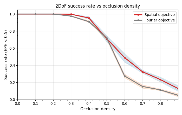
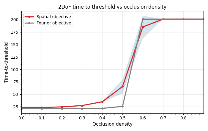
At low-to-mid occlusion densities the Fourier objective reaches the EPE threshold in fewer steps and with a flatter TTT curve — it converges more consistently rather than just faster on average. Success rates are comparable across all densities. Above roughly 50% density the zero-motion bias overwhelms the signal term regardless of domain, exactly as the theory predicts, with the spatial method failing slightly more gracefully.
The Fourier formulation makes the bias legible — instead of just “hurts at high density” you can read off exactly why and at what rate. The next post extends this to similarity motion, where the challenge turns out to be structural even before occlusion enters.
Until then!